4 Land Cover and Crop Classification Schemas for Agricultural Statistics
4.1 Introduction
Satellite imagery represents the most comprehensive data source for monitoring our environment, providing essential insights into global challenges. These images allow us to measure deforestation, crop production, food security, urban footprints, water scarcity, and land degradation. In recent years, adoption of open distribution policies by space agencies has made petabytes of Earth Observation (EO) data available. Experts now have access to repeated acquisitions over identical areas, resulting in time series that significantly improve our understanding of ecological patterns and processes [1]. Instead of selecting individual images from specific dates for comparison, researchers can now track changes continuously [2].
The raw data generated by EO satellites —pixels representing spectral reflectance— are meaningless without a rigorous interpretive framework. This framework is provided by Land Use and Land Cover (LULC) classification schemas. This chapter examines the critical role of LULC classification schemas in generating agricultural statistics from remote sensing data. It explores the conceptual distinction between land cover and land use, the utility of standardized hierarchical systems like the FAO Land Cover Classification System (LCCS), and the challenges posed by the dynamic nature of agricultural systems. We analyze the integration of modern technologies—including Satellite Image Time Series (SITS), big EO data, and machine learning—into classification frameworks. We argue that robust schema design is not merely a technical taxonomy but a critical semantic infrastructure ensuring data interoperability and statistical validity in the era of big Earth data.
4.2 Problem Statement
Remote sensing provides a synoptic view of agricultural landscapes, capturing electromagnetic reflectance that correlates with plant health, biomass, and moisture. Yet, a fundamental disconnect remains: satellites measure physical properties (spectral radiance), whereas policymakers require thematic information (crop type, yield, and land use intensity). This disconnect is bridged by the classification process, which assigns semantic labels to clusters of pixels. The efficacy of this process depends entirely on the design of the classification schema—the set of rules, definitions, and hierarchies that organize the complex reality of the landscape into discrete, quantifiable categories.
Consider how experts utilize EO data. Inputs typically consist of images with resolutions ranging from 5 to 500 meters, produced by satellites such as Landsat, Sentinel-1/2/3, and CBERS-4. To extract information, methods are applied to assign a label (e.g., ‘grasslands’) to each pixel. However, labels can represent either land cover or land use. Land cover is the observed biophysical cover of the Earth’s surface, while land use describes socio-economic activities [3]. Thus, ‘forest’ is a type of land cover, while ‘corn plantation’ is a type of land use. To support land classification, scientists have proposed ontologies and descriptive schemes [4]. This prompts the question: Are current classification systems suitable for representing land change when working with big data? If not, which concepts are needed, and how should they be applied?
A poorly designed schema can lead to conceptual confusion, where classes overlap (e.g., “Arable Land” vs. “Irrigated Land”) or fail to capture temporal dynamics (e.g., classifying a fallow field as “Bare Soil” rather than “Agricultural Land”). This chapter interrogates the design principles of LULC schemas, arguing that a shift toward temporally dynamic systems is essential for the future of agricultural statistics. To support this view, we consider concepts used in image time series analysis, demonstrating their relation to event recognition—a concept not representable in static schemas such as FAO’s LCCS [4]. To improve the theory behind big data, we introduce elements of a phenology-based approach for land classification.
4.3 Land Cover and Land Use
To design an effective schema, one must first distinguish between the central concepts of Land Cover (LC) and Land Use (LU). While often used interchangeably in casual discourse, they represent distinct ontological domains in remote sensing and statistics.
Land Cover refers to the observed (bio)physical material on the Earth’s surface. It is an objective property directly observable by sensors (e.g., “Broadleaved Forest,” “Water Body,” or “Impervious Surface”). In contrast, Land Use refers to the socioeconomic function for which the land is managed. It is a subjective, human-centric attribute that often requires context beyond the spectral signature (e.g., “Commercial Forestry,” “Recreation Area,” or “Residential Zone”) [[5]][6][7].
The distinction between these concepts creates a semantic gap. For agricultural statistics, the primary interest is usually land use (e.g., “Is this land used for food production?”), yet remote sensing primarily detects land cover (e.g., “Is there vegetation here?”). This creates ambiguity; a field of wheat and a field of wild grass may have nearly identical spectral signatures, but their land use differs fundamentally (Agriculture vs. Natural Vegetation).
Furthermore, the relationship is rarely one-to-one. A single land use type, such as “Agricultural Land,” can manifest as multiple Land Covers depending on the season (e.g., “Vegetated,” “Bare Soil,” or “Water”). Conversely, a single land cover can serve multiple land uses; a grassy area could be a “Pasture,” a “Park,” or an “Airfield” [8]. Consequently, effective classification schemas for agricultural statistics must be hybrid or coupled systems. These systems must explicitly map the relationships between detectable LC classes and inferred LU classes, often leveraging ancillary data—such as temporal patterns or proximity to infrastructure—to resolve ambiguities.
4.4 Classification Systems for Earth observation Data
The act of classification raises philosophical questions dating back to Aristotle. We impose a priori conceptions of reality onto the world; what we observe is forced to fit our established categories. While language provides words to describe external reality, geographical terms such as “forest” and “river” are inherently imprecise and context-dependent [11].
In Earth observation, these semantic constraints become rigid technical limitations. Experts define a closed set of possible object descriptions (e.g., “Forest,” “Pasture”), and individual pixels are labeled via visual or automated interpretation to fit these buckets. A prominent example is the Intergovernmental Panel on Climate Change (IPCC), which restricts top-level land classes for greenhouse gas inventories to just six categories: “Forest,” “Cropland,” “Grassland,” “Wetlands,” “Settlements,” and “Others.”
This approach is reductionist. Sasaki and Putz [12] argue that the simplistic IPCC base classes induce erroneous assessments for ecological and biodiversity conservation. These classes exemplify the ontological mismatch that occurs when pre-conceived, rigid rules collide with the heterogeneous reality of the world’s ecosystems.
4.5 The Evolution of Classification Systems
The history of Land Use and Land Cover (LULC) classification reflects a tension between the need for local specificity and the necessity of global standardization. Early efforts, such as the seminal Anderson Classification System (1976) developed by the USGS, were primarily a priori systems. In this approach, classes are defined before data collection begins, creating a rigid tree of mutually exclusive categories (e.g., Level I: Agriculture \(\rightarrow\) Level II: Cropland). While the Anderson system standardized mapping in the United States, it suffers from intrinsic rigidity. If a landscape feature does not fit into pre-defined boxes—for example, an agroforestry system that is both “Forest” and “Agriculture”—the system fails. This forces the classifier to make arbitrary decisions, introducing bias and reducing statistical reliability.
Recognizing the limitations of rigid legends, the Food and Agriculture Organization (FAO) and UNEP developed the Land Cover Classification System (LCCS). There are two main versions of LCCS: LCCS version 2, which is a modular, hierarchical a priori classification system [13], and LCCS version 3, which is uses an a posteriori approach. Since LCCS2 remains widely used by remote sensing experts, we describe it first before moving into LCCS3.
4.5.1 LCCS version 2
The stated aim of LCCS is “to provide a consistent framework for the classification and mapping of land cover” [13]. At its highest level, LCCS2 divides the world into eight major land cover types based on three criteria: presence of vegetation, edaphic conditions, and artificiality of cover:
- Cultivated and managed terrestrial areas.
- Natural and semi-natural terrestrial vegetation.
- Cultivated aquatic or regularly flooded areas.
- Natural and semi-natural aquatic or regularly flooded vegetation.
- Artificial surfaces and associated areas.
- Bare areas.
- Artificial water bodies, snow, and ice.
- Natural water bodies, snow, and ice.
Specialization of top-level LCCS2 classes uses properties such as life form, tree height, and vegetation density, setting pre-defined limits (e.g., “tree height > 10 meters”). These subdivisions are ad hoc and application-dependent, leading to a combinatorial explosion with dozens or even hundreds of subclasses [14]. Such high expressive power can lead to incompatible LCCS2-based class hierarchies [15].
While LCCS2 underpins major products like GLOBCOVER [16] and ESA CCI Land Cover [17], it makes assumptions that limit its utility for big data and modern applications:
- LCCS2 describes land properties based only on land cover types, disregarding land use. For example, LCCS2 does not distinguish “Pasture” from “Natural Grasslands”; it labels both as herbaceous land cover types.
- The LCCS2 hierarchy uses hard boundaries between its subclasses. At each level of the hierarchy, properties of subclasses use fixed values (e.g., “sparse forests have between 10% and 30% of trees”). Real-world class boundaries do not fit into such strict definitions. When doing data analysis with machine learning, boundaries between classes are data-dependent and cannot be set a priori [18].
- Classification in LCCS2 has no temporal reference. LCCS2 assumes that subtype properties (e.g., percent of tree cover) are detectable at the moment of classification. These properties do not refer to past or future values. Land use and land cover types whose values require time references (e.g., “forest land cleared in the last decade”) are not representable in LCCS2.
For example, the UNFCCC Reduction of Emissions by Deforestation and Degradation initiative (REDD+) requires capturing forest dynamics [19]. Static and rigid definitions of “Forest” used by LCCS cannot represent concepts such as `forest degradation’ [20]. Forest degradation happens when a natural forest loses part of its biodiversity and its tree cover. It is not a stable state but an intermediary situation that can lead to different medium-term outcomes. One can restore a degraded forest; degradation may continue and lead to complete loss of forest cover. Whatever the case, LCCS2 lacks explicit temporal information to capture forest degradation and thus support initiatives such as REDD+. Consequently, LCCS2 is ill-suited for many critical applications of EO data.
4.5.2 LCCC version 3
Version 3 of LCCS introduces an a posteriori approach. Instead of forcing land into pre-named buckets, the system provides a set of independent diagnostic criteria (classifiers) that can be combined to describe any land cover feature. The system uses LCML (Land Cover Metalanguage) —formalized by the ISO 19144-2 standard— that acts as a grammar for building classes. This criteria includes a dichotomous phase which broad splits (e.g., Vegetated vs. Non-Vegetated) and a modular-hierarchical phase with detailed descriptors (e.g., Life Form, Leaf Type, Stratification). Thus, a key difference between LCCS3 and LCCS2 is the possibility for users to build specific classes targeted to their applications.
The purpose of the LCML standard is to be a grammar for building classes, ensuring that different schemas can be converted to each other. LCCS3 argues for domain ontologies based on a common foundational ontology. Consider the case of experts in Spain and Poland that develop of a classification schema for permanent tree crops independently. The class “Tree Crop” would be specialized in “Olive Grove” in Spain and “Apple Orchard” in Poland. To ensure interoperability, experts in Spain and Poland would have to agree that the “Tree Crop” class belongs to a common hierarchy such as Terrestrial > Cultivated > Woody > Tree Crop. This communality allows for cross-walking. Different countries can maintain their specific local classes (e.g., “Olive Grove” vs. “Apple Orchard”) while still allowing external users to aggregate both into a standardized “Tree Crop” category for global reporting. Each application would develop a classification schema based on the same basic ontology, allowing these schemas to be interoperable.
However, building interoperable ontologies requires that each concept used in each specific ontology is unambiguous [21]. Janowicz et al. [22] recognize that “geographical concepts are situated and context-dependent, can be described from different, equally valid, points of view, and ontological commitments are arbitrary to a large extent”. Some experts may use the same class name with different meanings, thus making interoperability impossible.
Take the concept of “Forest”, which is inherently ambiguous [23]. UNFCCC defines a “Forest” as “an area with 10% to 30% cover of plants that grow to 2 to 5 metres high at maturity”. This definition does not capture the loss of carbon and ecosystem services when a forest ecosystem is severely degraded or replaced by plantations. The resulting cover would still be called “Forest” according to UNFCCC [12]. FAO considers that a forest may be temporarily devoid of trees, a condition that is impossible to measure using single-date images. Biodiversity researchers and timber companies use different definitions of forest [23]. In Northern European countries such as Finland, most forest areas are managed, sometimes in 50 to 100-year cycles. By contrast, in Brazil it is important to measure how much native tropical forest areas are kept intact, because of their role in preserving biodiversity and storing carbon. Furthermore, many tropical countries also have considerable areas of dry forests, which are completely different ecosystems than moist broadleaf forests.
Consider a group of experts from different countries that want to design a geospatial ontology that will achieve full interoperability in their map products. Starting from the top-level concept of “Forest”, what comes next? Timber companies would like to introduce the dichotomies “Cultivated/Natural Forest” and “Unmanaged/Managed Forest”, while ecologists would want to distinguish between “Humid/Dry Forest”, “Broadleaf/Needleleaf Forest” and “Degraded/Preserved” forest. It is doubtful that the experts could agree on a single ontology that would fit such diverse purposes and interests. Most likely, each application would have its own fit-for-purpose ontology expressed in the LCML metalanguage.
Therefore, because of the ad-hoc nature of the problems being addressed by EO data analysis, the ontologies produced by LCCS3 may not be translatable. In fact, direct conversion between different geospatial ontologies is only possible if they follow a strict hierarchical approach and avoid ambiguous definitions [24] [21]. Despite relevant efforts by FAO to promote LCCS3, its use remains limited in the community.
4.6 Specific Challenges in Agricultural Classification
The implementation of these schemas faces several hurdles that require careful design considerations.
In many advanced agricultural systems, the land cover changes every year (e.g., Maize in Year 1, Soybeans in Year 2). A static map labeled “Maize Field” is obsolete within 12 months. With the increased availability of methods for classification of image time series, we are moving toward dynamic land use dystems. The schema must classify the rotation pattern (e.g., “Corn-Soy Rotation”) rather than just the instantaneous cover, as this is more stable and predictive for long-term statistics.
Intercropping (growing two crops simultaneously) and integrated production systems (mixing pasture with natural vegetation) defy mutually exclusive classification. In principle, a LUCC class could be defined as having two distinct layers, Woody Vegetation (Trees) with 40% cover, and Herbaceous Vegetation (Pasture) with 60% cover. In that case, statisticians could account for both the timber/fruit production of the trees and the grain production of the understory, preventing the under-reporting of either commodity. However, there is a major challenge of identifying these classes in remote sensing images.
Another hard challenge for remote sensing classification is separating “Pasture” from “Natural Grassland”, since a grazed pasture often looks spectrally identical to a natural savanna. To address this problem, experts need to combine image time series, multispectral bands and adequate resolution images. Image time series capture the different seasonal variations of herbaceous pasture and natural savannas. Multispectral bands, such as those available in the Sentinel-2 satellites, improve such discrimination. Recent analysis shows that Sentinel-2 image time series provide a better discrimination than Planet images with higher spatial resolution but lower spectral discrimination [25].
4.7 Design Principles for LUCC Schemas for Agricultural Statistics
Designing a schema specifically for agricultural statistics requires addressing the unique characteristics of farming systems, while also considering the interrelation between natural and human-shaped lands. The first principle is that of aggregation. Agricultural statistics are reported at multiple scales. A local official needs to know the acreage of “Winter Wheat,” while a national minister needs “Cereals,” and a global analyst needs “Arable Land.” A robust schema should be strictly hierarchical. The boundaries of lower-level classes (children) must be perfectly contained within the boundaries of higher-level classes (parents). An example of a possible hierarchy:
- Level 1: Agricultural Land
- Level 2: Annual Crops
- Level 3: Cereals
- Level 4: Maize
This hierarchy allows for collapsing. If a satellite sensor cannot distinguish between Wheat and Barley due to cloud cover, the classification can move to Level 3 (“Cereals”) without losing statistical validity. One example of multi-level LUCC schema is provided by the Chile use case in this Handbook, “Crop Classification and Land Use Mapping in Chile”. Target crops are a wide variety of horticultural and field crops relevant to Chile’s export-oriented agriculture (e.g., fruit trees, vineyards, annual crops).
The authors of the Chilean report developed a new classification scheme that maintains a hierarchical structure—balancing technical limitations with institutional requirements — while placing significantly greater emphasis on the phenological dimension. This multi-level structure enables a more precise thematic breakdown (e.g., winter crops, successive crops, fallow land) by integrating observable variables from vegetation curves, such as NDVI. Crucially, the scheme recognizes the dynamic nature of these classes, replacing a fixed-coverage approach with a temporally explicit one
Since agriculture is inherently dynamic, a static map is often insufficient. Thus, the class definitions must often include a temporal component. One example is the distinction between “Fallow Land” and “Abandoned Land”. “Fallow” implies a temporary rest within an agricultural cycle, whereas “Abandoned” implies a cessation of use. When looking to such regions at a single point of time, spectrally both look like “Bare Soil”. For this reason, the use of image time series has become a recommended practice.
4.8 The Key Role of Time Series
The advent of open, high-resolution Earth Observation (EO) big data enables a paradigm shift in remote sensing for agricultural statistics. Moving beyond the traditional analysis of static “snapshots”, the field is embracing Satellite Image Time Series (SITS) as the standard for monitoring. This shift is not merely technological; it is ontological. It changes how we perceive the landscape—not as a fixed mosaic of objects, but as a dynamic arena of events. Given the temporal richness of modern EO data renders traditional, static classification schemas obsolete. Thus, we argue toward temporally explicit, hierarchical classification systems that prioritize phenology and cropping sequences over simple cover types.
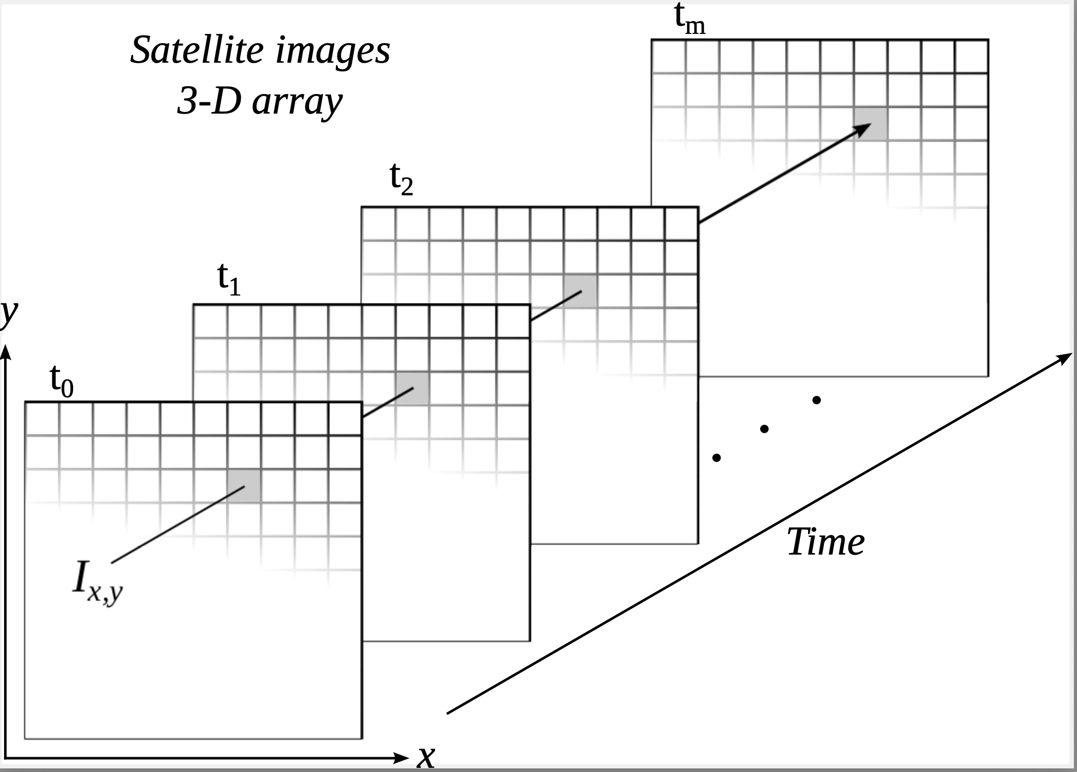
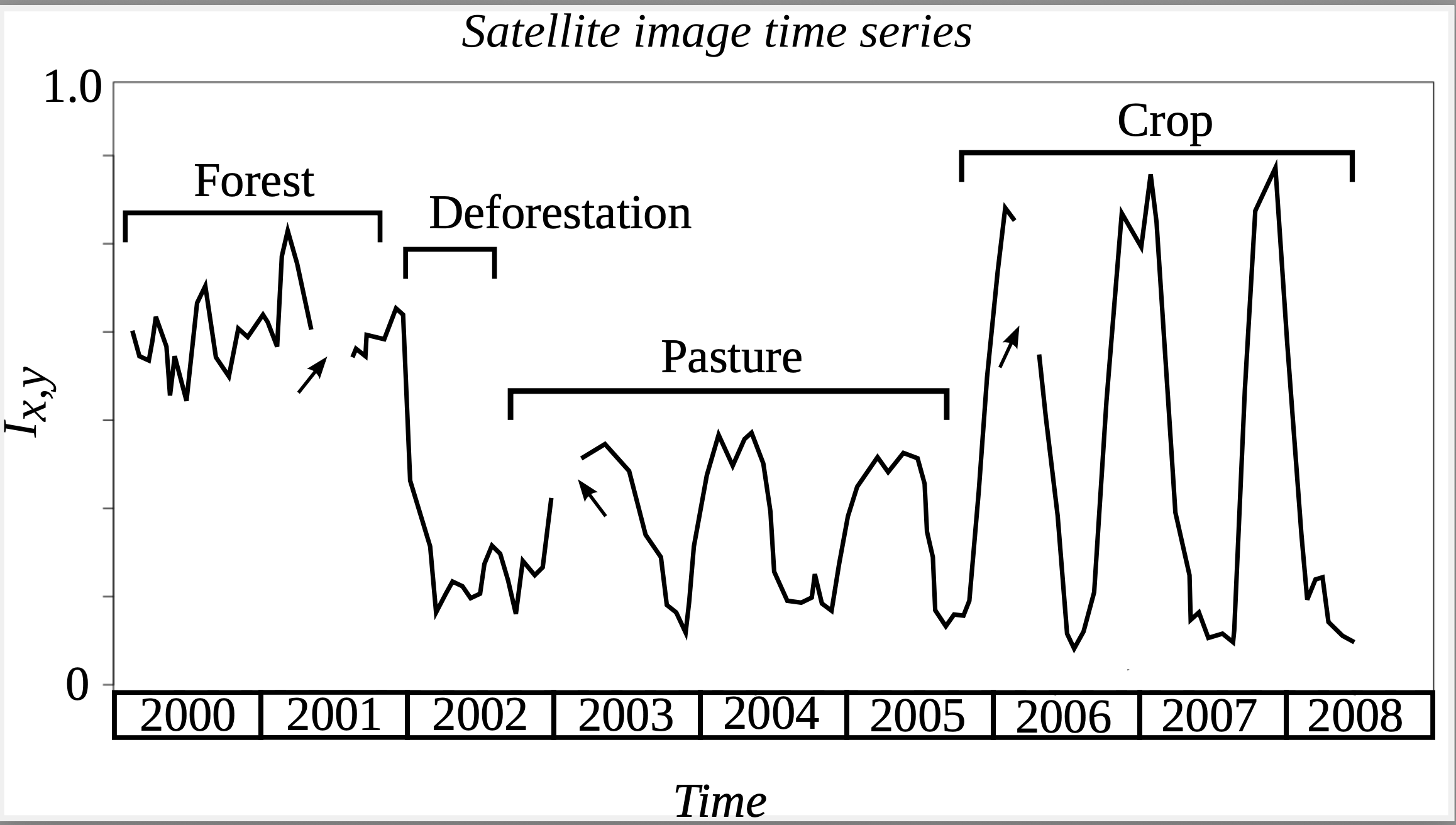
Since remote sensing satellites revisit the same place, we can calibrate their images so that measures of the same place at different times are comparable (Figure 4.1). These observations can be organized so that each measure from the sensor maps to a three-dimensional array in space-time. From a data analysis perspective, each pixel location \((x, y)\) at consecutive times, \(t_1,...,t_m\), makes up a satellite image time series (SITS), such as the one in Figure 4.2. From these time series, we can extract land-use and land-cover change information. In Figure 4.2, after the forest was cut in 2002, the area was used for cattle raising (pasture) for three years, during 2002 to 2008, then turned into cropland.
For decades, the production of agricultural statistics via remote sensing was constrained by data scarcity. Analysts relied on “best-available” cloud-free composites—single images or seasonal mosaics—to classify land cover. In this “space-first” paradigm, a pixel was classified based on its spectral signature at a specific moment in time.
However, agriculture is inherently defined by time. A field is not simply “bare soil” or “vegetated”; it is a dynamic system that transitions from sowing to emergence, maturation, senescence, and harvest. A static image taken in May might correctly identify a field as “vegetated,” but it cannot distinguish between a winter crop reaching maturity and a summer crop just emerging. Furthermore, single-date imagery fails to capture the complexity of intensification, such as double-cropping systems (e.g., Soybean-Maize rotations), which are critical for estimating total production and understanding food security.
The resulting statistics often suffered from significant uncertainties. Confusing spectrally similar crops (e.g., wheat vs. barley) or failing to detect fallow periods led to errors in acreage estimation. Today, with the availability of dense time series from constellations like Sentinel-2 and Landsat, we have moved to a “time-first” paradigm. The core advantage of SITS is its ability to capture land surface phenology. Every crop type has a unique temporal signature—a “fingerprint” defined by its life cycle. We no longer look at a photo of the land; we watch the “movie” of the growing season. This capability demands a fundamental rethinking of how we design the legends and schemas that categorize our world.
4.9 Using Time Series for Designing LUCC Classification Schemas
To represent change in geographical space, GIScience authors distinguish between objects (continuants) and events (occurrents) [30]. Continuants refer to entities that “endure through time even while undergoing different sorts of changes” [27]. The Amazon Forest and the city of Brasilia are continuants. Occurrents happen in a well-defined period and may have different stages during this time. Cutting down a forest area, cultivating a crop in a season, and building a road are occurrents.
Atemporal classification systems such as LCCS2 refer only to properties of continuants (fields and objects). One can state facts such as “this area has 30% forest cover” using LCCS2, but cannot assert that “this area lost 70% of its forest in the last two years”. To convey change, classification systems for big data need to include events [31]. In what follows, we discuss concepts used in the analysis of satellite image time series. These time series are extracted from organized collections of Earth observation data covering a geographical area in regular temporal intervals.
Using image time series allows for the detection of land use events rather than just land cover states. We can identify plowing (sudden drop in reflectance), irrigation (sustained greenness during dry periods), and multi-cropping practices. However, to leverage this power, our classification schemas must be able to describe these complex temporal events. Traditional schemas, such as LCCS2, were built around static, mutually exclusive categories: “Forest”, “Water”, “Urban”, “Cropland”. In these systems, a pixel belongs to one class for the duration of the map’s validity (usually a year). Using SITS, we can improve on this static classification systems.
In a static map, “Fallow” is a confusing class. Is it bare soil? Is it grassland? In reality, fallow is a temporal state, not a permanent cover type. A field may be bare soil in January, fallow with spontaneous grass in March, and planted with Maize in November. A static schema forces the analyst to simplify this reality into a single label, losing critical information about land use intensity. A SITS-oriented schema treats “Fallow” as a phase within a cropping cycle, not a rigid land cover class.
Global food security relies heavily on intensification—growing two or even three crops on the same plot within a year (e.g., widespread Soy-Corn rotations in Brazil or Rice-Rice systems in Vietnam). A schema that simply lists “Soybean” and “Maize” as separate classes is insufficient for these regions. If a pixel contains both during the year, classifying it as the “main” crop ignores the second harvest, biasing production statistics. Also, labeling it “Mixed Agriculture” is vague and unhelpful for yield estimation.
As an alternative, SITS enables trajectory-based schemas. The class is no longer a single crop but a cropping sequence, e.g., (a) Soybean (Single crop); (b) Soybean - Maize (Double crop); (c) Soybean - Cotton (Double crop). This approach makes the schema temporally explicit. It acknowledges that the identity of the land changes throughout the timeline.
Designing these schemas requires defining the temporal unit of analysis. Are we classifying the calendar year (January to December) or the agricultural year (sowing to harvest)? SITS forces statisticians to align the classification window with the biological reality of the crop. For example, in the Southern Hemisphere, a crop season spans across two calendar years (sown in late 2024, harvested in early 2025). A rigid calendar-year schema would slice the crop phenology in half, destroying the signal. Modern LUCC schemas must be flexible enough to encompass the full phenological cycle.
4.10 Conclusion
In this chapter, we discuss the challenge of supporting big data analysis with sound theory. We argue that time series analysis, including pattern matching, trend analysis, break detection, and time series classification, are subtypes of event recognition. When doing continuous monitoring of land change, it is not advisable to use LCCS2 and similar approaches. Instead of identifying classes such as “Forest” or “Grassland”, data analysis methods need to recognize events such as “this area was a forest from 2000 to 2010, then it was deforested in 2011, and turned into grasslands from 2011 to 2020”. When doing continuous monitoring, event recognition replaces object identification as the purpose of land classification.
The emphasis on event recognition has significant consequences for the design of algorithms and classification systems for big data. In particular, machine learning is not a panacea. Continuous monitoring of land dynamics using remote sensing data differs from applications such as spam filters, automatic translation, and object detection. Land systems do not change overnight. There is a period of transition for land cover conversion. Depletion of natural resources such as forests and wetlands can take place over months or even years. Monitoring subtle land transitions is crucial for protecting our environment. Thus, machine learning methods need to be adapted to work with satellite image time series.
Most algorithms for big EO data analysis use techniques that have proven useful in other problems. However, monitoring natural resources is more complex than detecting spam emails or playing chess. While machine learning and pattern analysis are useful, there is still much to be done to build sound theories for dealing with big EO data. Long-term progress will depend on a new generation of methods that combine machine learning with functional ecosystem models. A better theoretical basis is essential for algorithms that extract information from petabytes of free EO data. This new generation of combined methods will allow a better understanding of the processes that drive landscape dynamics.
References
[1]
V. J. Pasquarella, C. E. Holden, L. Kaufman, and C. E. Woodcock, “From imagery to ecology: Leveraging time series of all available LANDSAT observations to map and monitor ecosystem state and dynamics,” Remote Sensing in Ecology and Conservation, vol. 2, no. 3, pp. 152–170, 2016, doi: 10.1002/rse2.24.
[2]
C. E. Woodcock, T. R. Loveland, M. Herold, and M. E. Bauer, “Transitioning from change detection to monitoring with remote sensing: A paradigm shift,” Remote Sensing of Environment, vol. 238, p. 111558, 2020, doi: 10.1016/j.rse.2019.111558.
[3]
A. Comber, “The separation of land cover from land use using data primitives,” Journal of Land Use Science, vol. 3, no. 4, pp. 215–229, 2008, doi: https:/doi.org/10.1080/17474230802465173.
[4]
M. Herold, R. Hubald, and A. Di Gregorio, “Translating and evaluating land cover legends using the UN Land Cover Classification System (LCCS),” GOFC-GOLD Florence, Italy, 2009.
[5]
O. Ahlqvist, D. Varanka, S. Fritz, and K. Janowick, Eds., Land Use and Land Cover Semantics: Principles, Best Practices, and Prospects. CRC Press, 2017.
[6]
A. Comber, P. Fisher, and R. Wadsworth, “What is Land Cover?” Environment and Planning B: Planning and Design, vol. 32, no. 2, pp. 199–209, 2005, doi: 10.1068/b31135.
[7]
A. J. Comber, R. A. Wadsworth, and P. F. Fisher, “Using semantics to clarify the conceptual confusion between land cover and land use: The example of forest,” Journal of Land Use Science, vol. 3, no. 2–3, pp. 185–198, 2008.
[8]
A. J. Comber, P. F. Fisher, and R. A. Wadsworth, “Land cover: To standardise or not to standardise? Comment on ‘Evolving standards in land cover characterization’ by Herold et al.” Journal of Land Use Science, vol. 2, no. 4, pp. 283–287, 2008, doi: 10.1080/17474230701786000.
[9]
B. Smith and D. M. Mark, “Geographical categories: An ontological investigation,” International Journal of Geographical Information Science, vol. 15, no. 7, pp. 591–612, 2001, doi: 10.1080/13658810110061199.
[10]
B. Smith and D. M. Mark, “Do Mountains Exist? Towards an Ontology of Landforms,” Environment and Planning B: Planning and Design, vol. 30, no. 3, pp. 411–427, 2003, doi: 10.1068/b12821.
[11]
D. M. Mark and A. G. Turk, “Landscape Categories in Yindjibarndi: Ontology, Environment, and Language,” in Spatial Information Theory. Foundations of Geographic Information Science, 2003, pp. 28–45, doi: 10.1007/978-3-540-39923-0_3.
[12]
N. Sasaki and F. E. Putz, “Critical need for new definitions of ‘forest’ and ‘forest degradation’ in global climate change agreements,” Conservation Letters, vol. 2, no. 5, pp. 226–232, 2009, doi: 10.1111/j.1755-263X.2009.00067.x.
[13]
A. Di Gregorio, “Land Cover Classification System - Classification concepts Software version 3,” FAO, 2016.
[14]
M. Herold et al., “A joint initiative for harmonization and validation of land cover datasets,” IEEE Transactions on Geoscience and Remote Sensing, vol. 44, no. 7, pp. 1719–1727, 2006, doi: 10.1109/TGRS.2006.871219.
[15]
L. J. M. Jansen, G. Groom, and G. Carrai, “Land-cover harmonisation and semantic similarity: Some methodological issues,” Journal of Land Use Science, vol. 3, no. 2–3, pp. 131–160, 2008, doi: 10.1080/17474230802332076.
[16]
O. Arino et al., “GlobCover: ESA service for global land cover from MERIS,” in 2007 IEEE International Geoscience and Remote Sensing Symposium, 2007, pp. 2412–2415, doi: 10.1109/IGARSS.2007.4423328.
[17]
W. Li, P. Ciais, N. MacBean, S. Peng, P. Defourny, and S. Bontemps, “Major forest changes and land cover transitions based on plant functional types derived from the ESA CCI Land Cover product,” International Journal of Applied Earth Observation and Geoinformation, vol. 47, pp. 30–39, 2016, doi: 10.1016/j.jag.2015.12.006.
[18]
T. Hastie, R. Tibshirani, and J. Friedman, The Elements of Statistical Learning. Data Mining, Inference, and Prediction. New York: Springer, 2009.
[19]
E. Corbera and H. Schroeder, “Governing and implementing REDD+,” Environmental Science & Policy, vol. 14, no. 2, pp. 89–99, 2011, doi: 10.1016/j.envsci.2010.11.002.
[20]
F. E. Putz and K. H. Redford, “The Importance of Defining ‘Forest’: Tropical Forest Degradation, Deforestation, Long-term Phase Shifts, and Further Transitions,” Biotropica, vol. 42, no. 1, pp. 10–20, 2010, doi: 10.1111/j.1744-7429.2009.00567.x.
[21]
F. Fonseca, G. Camara, and A. M. Monteiro, “A Framework for Measuring the Interoperability of Geo-Ontologies,” Spatial Cognition & Computation, vol. 6, no. 4, pp. 309–331, 2006, doi: 10.1207/s15427633scc0604_2.
[22]
K. Janowicz, S. Scheider, T. Pehle, and G. Hart, “Geospatial semantics and linked spatiotemporal data – Past, present, and future,” Semantic Web, vol. 3, no. 4, pp. 321–332, 2012, doi: 10.3233/SW-2012-0077.
[23]
R. L. Chazdon et al., “When is a forest a forest? Forest concepts and definitions in the era of forest and landscape restoration,” Ambio, vol. 45, no. 5, pp. 538–50, 2016, doi: 10.1007/s13280-016-0772-y.
[24]
M. Herold, P. Mayaux, C. E. Woodcock, A. Baccini, and C. Schmullius, “Some challenges in global land cover mapping: An assessment of agreement and accuracy in existing 1 km datasets,” Remote Sensing of Environment, vol. 112, no. 5, pp. 2538–2556, 2008, doi: 10.1016/j.rse.2007.11.013.
[25]
J. P. S. Werner et al., “Mapping Integrated Crop–Livestock Systems Using Fused Sentinel-2 and PlanetScope Time Series and Deep Learning,” Remote Sensing, vol. 16, no. 8, p. 1421, 2024, doi: 10.3390/rs16081421.
[26]
M. Picoli et al., “Big earth observation time series analysis for monitoring Brazilian agriculture,” ISPRS Journal of Photogrammetry and Remote Sensing, vol. 145, pp. 328–339, 2018, doi: 10.1016/j.isprsjprs.2018.08.007.
[27]
P. Grenon and B. Smith, “SNAP and SPAN: Towards Dynamic Spatial Ontology,” Spatial Cognition & Computation, vol. 4, no. 1, pp. 69–104, 2004, doi: 10.1207/s15427633scc0401_5.
[28]
A. Galton, “Fields and Objects in Space, Time, and Space-time,” Spatial Cognition & Computation, vol. 4, no. 1, pp. 39–68, 2004, doi: 10.1088/1748-9326/6/4/04400510.1207/s15427633scc0401_4.
[29]
A. Galton, “Experience and History: Processes and their Relation to Events,” Journal of Logic and Computation, vol. 18, no. 3, pp. 323–340, 2008, doi: 10.1088/1748-9326/6/4/04400510.1093/logcom/exm079.
[30]
M. Worboys, “Event-oriented approaches to geographic phenomena,” International Journal of Geographical Information Science, vol. 19, no. 1, pp. 1–28, 2005, doi: 10.1080/13658810412331280167.
[31]
G. Camara, “On the semantics of big Earth observation data for land classification,” Journal of Spatial Information Science, vol. 2020, no. 20, pp. 21–34, 2020, doi: 10.5311/JOSIS.2020.20.645.