23 Crop Statistics using Weighted Area Estimators
23.1 Introduction
Accurate and timely availability of agricultural production data is crucial for international market transparency and, therefore for ensuring global food security. Traditionally, these data are obtained through reporting, agricultural censuses, and field surveys [1]. However, natural or human-induced catastrophes may temporarily or for an extended period of time disrupt reporting and ground data collection possibilities. In such cases, these data can be complemented, or supplemented, with satellite remote sensing [2], which offers a cost-efficient means to monitor crops consistently across large spatial and temporal scales.
A first step towards remote-sensing based agricultural production assessment is crop type mapping for crop planted area estimation. Accurate crop-type identification from satellite imagery remains challenging in large, heterogeneous agricultural regions characterized by diverse crop types and variable field sizes [3]. It requires high-quality satellite data, representative ground-truth samples for training, probabilistically selected validation datasets, and high-performance computing infrastructure for large-scale processing. Very often, crop area is estimated from a map using the pixel-counting estimator: multiplying pixel area by the total number of pixels belonging to a class of interest. Although widely used, this estimator is intrinsically biased because it integrates classifier omission, commission, and edge pixel errors [4] [5]. In contrast, sample-based estimators of area rely on a probabilistic reference data sample, where a map can be used for stratification to estimate area and corresponding uncertainties [6]. Recent studies have demonstrated the benefits of integrating these approaches to generate consistent crop area estimates at the national scale, for soybean in the United States [3], Argentina [7], and South America [8]; wheat in Pakistan [9]; and sunflower in Ukraine [10]. This integration not only enhances the reliability of agricultural statistics but also supports timely decision-making for food security and disaster response. However, obtaining high-quality field-based observations remains a major challenge, as ground surveys are often costly, time-consuming, and, in some cases, infeasible due to armed conflicts, government restrictions, or logistical issues. When ground visits are prevented or too expensive, remote-sensing imagery interpretation is a viable alternative for reference data collection. This approach has been successfully applied in conflict contexts in Ukraine [10] [11]; Ethiopia (Tigray region) [12]; Sudan [13]; and Syria [14] but also in large-scale institutional surveys such as the Land Use and Coverage Area Frame Survey where 200,000 sample units were annotated with remote sensing imagery interpretation in the 2022 edition [15].
The primary objective of this chapter is to demonstrate an end-to-end, remote sensing-only framework for sample-based crop planted area estimation, without field visits. Based on work from [17], this chapter focuses on the use case of sunflower planted area estimation in Ukraine in 2023. This use case is particularly relevant under several aspects: (i) Monitoring sunflower is critical for markets and policy: Ukraine is one of the largest global producers of sunflower, a highly profitable cash crop; (ii) Sunflower production has a significant impact on soil degradations due to violations of crop rotation policies; (iii) Between March 3rd, 2022 and August 18th, 2025 martial Law №2115-IX suspended mandatory reporting for agricultural holdings (85% of producers) and interrupted surveys of small holder farmers (15% of producers) in Government-controlled territories. Meanwhile, in Russian-held territories, no more agricultural statistics were published from the onset of the full-scale war in February 2022. With the war preventing ground access, remote sensing offered a viable alternative for tracking sunflower planted area to complement official statistics in Ukraine-controlled regions and to compensate for the absence of data in Russian-held regions.
23.2 Data
23.2.1 Remote Sensing datasets
In this study, we utilized the C-band Sentinel-1 (S1) data in Interferometric Wave (IW) mode in VV and VH mode which have a temporal revisit of 12 days. The dataset selected was Ground Range Detected (S1_GRD) Level 1, pre-processed in Google Earth Engine (GEE) using the S1 toolbox [18]. The σ◦ values were converted to decibels (dB) via log scaling (10*log10σ◦). We also utilized Sentinel-2 (S2) harmonized surface reflectance products available on GEE (COPERNICUS/S2_SR_HARMONIZED). The Level-2 S2 dataset was pre-processed for atmospheric correction, and the scenes with cloud cover of >30% were filtered out using the image property of “CLOUDY_PIXEL_PER-CENTAGE” to avoid any potential cloud contamination.
23.2.2 Cropland mask
The European Space Agency (ESA) WorldCover 10 m 2020 product available on GEE (“ESA/WorldCover/v100”) was utilized for masking non-cropland region [19]. This land cover map provides a global land cover map for 2020 at 10-m resolution based on Sentinel-1 and Sentinel-2 data. The WorldCover product comes with 11 land cover classes with “Cropland” class (ID = 40) used for masking non-cropland areas.
23.3 Methods
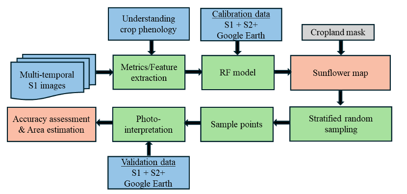
When no ground-reference data can be collected, the first step towards crop mapping and crop planted area estimation is identifying biophysical or phenological traits that distinguish the target crop (here sunflower) from other crop types, and how those specific traits translate into remote-sensing interpretable signals. Once crop-specific signals are well understood, the base knowledge for generating a stratifier for area estimation is available, and the target crop can be classified. After classification, the map is used within the stratified random sampling design,and sample units are annotated with remote sensing imagery, recognizing the crop-specific signals. Unbiased estimators of area can finally be applied to derive areas and uncertainties. This conceptual workflow was applied to the sunflower area estimation use case in Ukraine. The overall methodological approach is shown in Figure 23.1 and is composed of three modules:(i) Understanding sunflower phenology and recognizing sunflower on Sentinel-1/2 imagery; (ii) Random forest classification model for sunflower mapping; (iii) Stratified random sampling following best recommended practices in [20], sample unit annotation, area, and uncertainty estimation.
23.3.1 Understanding sunflower phenology using S1 sensor
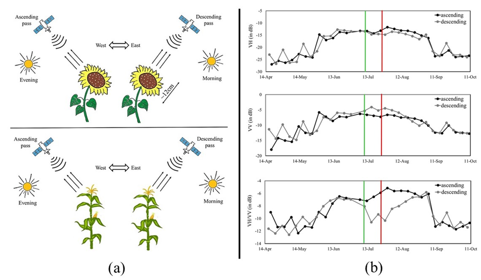
Sunflower exhibits several distinctive morphological and physiological traits, characterized by broad leaves, yellow capitula, which facilitate its discrimination from other summer crops such as maize and soybean (Figure 23.2) [16]. Another key feature of sunflower is heliotropism, the solar tracking of young leaves and buds. The plant follows the Sun from east to west during the day and reorients eastward at night through its circadian rhythm. Once flowering begins, this movement ceases, and the flower heads remain permanently oriented eastward (Figure 23.2), imparting a directional effect to the canopy.
These traits have direct implications for C-band SAR observations. S1, operating at ∼5.6 cm wavelength, is particularly sensitive to structural elements comparable in size to sunflower heads. Over Ukraine, S1’s sun-synchronous, right-looking antenna descends from north to south at approximately 04:00 UTC (07:00 local time) (Figure 23.2). During the flowering stage,when sunflower heads become fixed eastward, toward the descending pass, the canopy’s directional orientation enhances backscatter in the VV polarization and reduces the VH/VV ratio (Figure 23.2). This directional scattering effect, unique to sunflower, significantly improves their separability from other summer crops such as maize and soybean in Sentinel-1 descending orbit data.
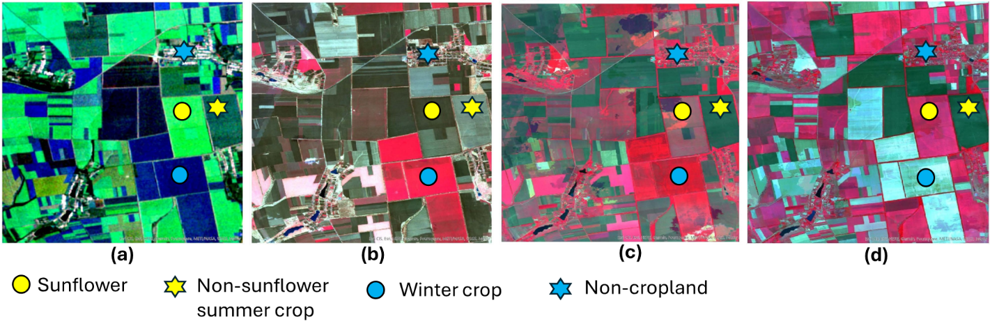
Recognizing sunflower in remote sensing imagery relies on its distinctive backscattering and spectral characteristics relative to other summer crops, particularly maize and soybean, during the flowering period. The pronounced directional effect of sunflower, captured by Sentinel-1 (S1) descending-orbit observations, manifests as elevated VV backscatter and reduced VH/VV ratios during summer months. To visualize these seasonal patterns, median S1 composites are generated for spring (March–May), summer (June–August), and autumn (September–November), assigning VV backscatter from each season to the red, green, and blue channels, respectively (Figure 23.3 (a)). In these composites, sunflower fields typically appear as bright neon-green patches, reflecting their strong summer backscatter response, whereas other summer crops exhibit more muted tones.
Complementary interpretation using Sentinel-2 (S2) optical imagery further enhances the ability to distinguish sunflower from other summer crops, winter crops and non-cropland. Bi-monthly S2 composites are created using the Near-Infrared (B8), Red (B4), and Green (B3) bands assigned to red, green, and blue channels, respectively, for March–April, May–June, and July–August (Figure 23.3 b–d). These composites highlight different crop phenological stages: winter crops dominate early-season imagery, while summer crops, including sunflower, become prominent in July–August, exhibiting high near-infrared reflectance and a distinct reddish hue. By combining the structural and directional information from S1 with the phenological and spectral cues from S2, sunflower fields can be effectively recognized and visually separated from other crops and land-cover types across Ukraine. Figure 23.3 exemplifies the sunflower recognition process based on remote sensing imagery interpretation with the corresponding Google Earth Engine (GEE) application.
23.3.2 Sunflower mapping
The sunflower mapping methodology follows [10] [17] and is based on the crop’s directional behavior. In the first step, a Random Forest (RF) model is calibrated using S1-derived metrics and randomly selected sunflower, non-sunflower cropland, and non-cropland photo-interpreted labels as described in Section 23.3. Non-cropland class of water, forest/vegetation, urban, and barren land was identified by integrating high-resolution Google Earth imagery over the S1 and S2 images. Calibration incorporates 42 multi-temporal metrics derived from S1 ascending and descending orbit data, which are processed separately to capture sunflower’s directional behavior characteristics.
The RF model is configured with 300 trees and default parameters for variables per split, minimum leaf population, and bag fraction. A two-phase classification strategy is implemented [17]. In the first stage, cropland is classified into six classes: sunflower, non-sunflower summer crops, winter crops, water, forest/vegetation, urban, and barren. In the second stage, all non-sunflower and non-cropland classes are aggregated into a single class, resulting in a binary map of sunflower and non-sunflower classes. To minimize misclassification with non-cropland areas, other land cover types are masked using the land cover map. Isolated pixels are filtered, and the final sunflower map is projected to the Albers equal area projection for subsequent analyses.
23.3.3 Sample-based crop area and accuracy estimation
Sample-based sunflower area and accuracy estimation follow the guidelines by [20] and use unbiased estimators for area and uncertainty estimation. The spatial extent of Ukraine was divided into Ukrainian and Russian-controlled territories according to the occupation line as of July 2023. Within each occupation status, sunflower, non-sunflower cropland, and non-cropland map classes are used as strata to draw samples in a simple random manner, where 20 × 20 m² resolution pixels are sample units. The required sample size (n) is calculated using the equation provided by [5] for estimating area and assessing the accuracy of sunflower maps and described in the “Map validation and use of maps for area estimation” chapter of this Handbook. Stratum weights and the corresponding number of sample units are presented in Table 23.1, per occupation status for 2023. The sample allocation deviates from a classical Neyman or proportional allocation design as the objective is to estimate precisely the sunflower area and reduce uncertainties for this stratum. Oversampling high-interest and undersampling low-interest strata is common in sample-based area estimation [20].
Each sample unit is then individually annotated based on the guidelines presented in Section 3.1. To avoid annotator’s bias, all sample units were annotated at least twice by independent labelers and experts in photo-interpretation of satellite imagery. If they disagree on a label, it should be reviewed collectively until a consensus is reached [21]. Following annotation, an area-weighted confusion matrix is constructed, based on which area, and map accuracies are computed along with uncertainties, following [20].
| Occupation status | Stratum | Wi | ni |
|---|---|---|---|
| Sunflower | 0.115 | 200 | |
| Ukrainian Government controlled | Cropland Non-Sunflower | 0.429 | 200 |
| Non-Cropland | 0.456 | 100 | |
| Sunflower | 0.056 | 200 | |
| Russian controlled | Cropland Non-Sunflower | 0.546 | 200 |
| Non-Cropland | 0.398 | 100 |
23.4 Results
Following the methodology presented in Section 23.3.1, we estimated sunflower planted areas based on a remote sensing-only framework, in Ukrainian and Russian-controlled territories in the 2023 season. The uncertainties are expressed as one standard error (SE). In Ukrainian-held territories, the sunflower area was estimated 5.99 ± 0.25 million hectares (Mha), while in Russian-held territories, 0.74 ± 0.06 Mha were planted to sunflower. The corresponding pixel-counted areas (biased estimator of areas) were 5.67 Mha and 0.60 Mha, respectively. The sunflower map for the 2023 season is shown in Google Earth Engine.
Table 23.2 presents area-weighted confusion matrices along with performance metrics: producer’s accuracy (PA), user’s accuracy (UA), and map overall accuracy (OA), per occupation status. In Government-controlled territories, classification performances for sunflower reflect high reliability of the map, with UA/PA close to or larger than 0.9. In Russian-held territories, sunflower mapping performance was still satisfactory with high UA (0.99 ± 0.01) while PA was lower at 0.80 ± 0.07. Those performance metrics illustrate the intrinsic bias of the pixel counting estimator, which would have integrated those classification errors into area estimates. Note that, lower map accuracy does not compromise the unbiasedness of the estimator of area, it simply results in higher variance (and therefore standard error) around area estimates [5] [20]. For instance, in this use case, the coefficient of variation (standard error/area) of the area estimate in Government-controlled territories is 4.7%, while in Russian-held regions, where map accuracy is lower, it is 8.1%.
| Reference | ||||||||
|---|---|---|---|---|---|---|---|---|
| SF | NSF-C | NC | UA | PA | OA | |||
| Gov. Cont. | Map | SF | 0.11 | 0.0002 | 0.00 | 0.97 ± 0.01 | 0.91 ± 0.04 | |
| NSF-C | 0.01 | 0.38 | 0.04 | 0.88 ± 0.02 | 0.96 ± 0.02 | 0.93 ± 0.01 | ||
| NC | 0.00 | 0.01 | 0.44 | 0.97 ± 0.02 | 0.91 ± 0.02 | |||
| Russ. Cont. | Map | SF | 0.056 | 0.0003 | 0.00 | 0.99 ± 0.01 | 0.80 ± 0.07 | |
| NSF-C | 0.014 | 0.442 | 0.09 | 0.81 ± 0.03 | 0.95 ± 0.02 | 0.87 ± 0.02 | ||
| NC | 0.00 | 0.024 | 0.374 | 0.94 ± 0.02 | 0.81 ± 0.03 |
23.5 Discussion
This chapter demonstrates the operational capability of SAR data for sunflower area estimation without relying on field observations at the country level. The directional behavior of sunflowers as detected by S1 data plays a crucial role in their identification and mapping.
By integrating a sampling-based approach in satellite-based crop mapping, the disparity between the sampling-based area and pixel-counting-based area is substantially reduced. To create the reference classification for labeling each sampling unit, a combination of S1 and S2 data from the Copernicus open archive, together with Google Earth imagery, provides a source of cost-free reference data equivalent to field observations required for sunflower identification (refer to Section 3.1). In this approach, the distinctive backscattering characteristics of sunflower observed by S1 facilitated the collection of higher-quality reference data for labelling compared to the classification-based map generation process, in accordance with the good practice recommendations of [20]. This approach is crop specific and should be applied cautiously to other crop types.
The proposed method has certain limitations, particularly in regions where only the S1 ascending orbit is available. [17] showed that in regions with only ascending orbit data, the model achieved lower accuracy compared to regions with both or only descending orbit coverage. Additionally, this approach relies on satellite acquisitions available till September or later months and therefore cannot be applied for early-season sunflower identification or area estimation. Furthermore, remote-sensing imagery interpretation to identify crop fields is based on expert knowledge of both SAR and optical data, which may vary among interpreters and across regions due to differences in crop cycles, crop types, and agroecological conditions. Therefore, caution should be exercised when applying this approach to other regions or smallholder farming systems, where sunflower (or another crop of interest) is not dominant and reference data collection becomes more challenging.
23.6 Conclusion
This chapter demonstrated a framework for sunflower-planted area estimation in Ukraine. The implemented approach relies solely on remote-sensing data to produce statistically sound, sample-based area estimates, where all reference data are derived through remote sensing imagery interpretation. At the core of this method lies the development of a deep understanding of the target crop by studying its unique spectral, structural, and phenological characteristics that distinguish it from other crops. Once this understanding is built, the reference data collection process with remote sensing imagery interpretation offers a low-cost, scalable, transparent and reliable alternative to ground surveys for crop planted area estimation.
References
[1]
J. Cotter, C. Davies, J. Nealon, and R. Roberts, “Area frame design for agricultural surveys,” Agricultural survey methods, pp. 169–192, 2010.
[2]
F. D. W. Witmer, “Remote sensing of violent conflict: Eyes from above,” International Journal of Remote Sensing, vol. 36, no. 9, pp. 2326–2352, 2015, doi: 10.1080/01431161.2015.1035412.
[3]
X.-P. Song et al., “National-scale soybean mapping and area estimation in the United States using medium resolution satellite imagery and field survey,” Remote Sensing of Environment, vol. 190, pp. 383–395, 2017, doi: 10.1016/j.rse.2017.01.008.
[4]
R. S. Chhikara, “Effect of mixed (boundary) pixels on crop proportion estimation,” Remote Sensing of Environment, vol. 14, no. 1, pp. 207–218, 1984, doi: 10.1016/0034-4257(84)90016-6.
[5]
S. Skakun, “The impact of map accuracy on area estimation with remotely sensed data within the stratified random sampling design,” Remote Sensing of Environment, vol. 326, p. 114805, 2025, doi: 10.1016/j.rse.2025.114805.
[6]
F. J. Gallego, “Remote sensing and land cover area estimation,” International Journal of Remote Sensing, vol. 25, no. 15, pp. 3019–3047, 2004, doi: 10.1080/01431160310001619607.
[7]
L. King et al., “A multi-resolution approach to national-scale cultivated area estimation of soybean,” Remote Sensing of Environment, vol. 195, pp. 13–29, 2017, doi: 10.1016/j.rse.2017.03.047.
[8]
X.-P. Song et al., “Massive soybean expansion in South America since 2000 and implications for conservation,” Nature Sustainability, vol. 4, no. 9, pp. 784–792, 2021, doi: 10.1038/s41893-021-00729-z.
[9]
A. Khan, M. C. Hansen, P. Potapov, B. Adusei, S. V. Stehman, and M. K. Steininger, “An operational automated mapping algorithm for in-season estimation of wheat area for Punjab, Pakistan,” International Journal of Remote Sensing, vol. 42, no. 10, pp. 3833–3849, 2021, doi: 10.1080/01431161.2021.1883200.
[10]
A. Qadir, S. Skakun, N. Kussul, A. Shelestov, and I. Becker-Reshef, “A generalized model for mapping sunflower areas using Sentinel-1 SAR data,” Remote Sensing of Environment, vol. 306, p. 114132, 2024, doi: 10.1016/j.rse.2024.114132.
[11]
S. Skakun, C. O. Justice, N. Kussul, A. Shelestov, and M. Lavreniuk, “Satellite Data Reveal Cropland Losses in South-Eastern Ukraine Under Military Conflict,” Frontiers in Earth Science, vol. 7, 2019, doi: 10.3389/feart.2019.00305.
[12]
H. Kerner et al., “How accurate are existing land cover maps for agriculture in Sub-Saharan Africa?” Scientific Data, vol. 11, no. 1, p. 486, 2024, doi: 10.1038/s41597-024-03306-z.
[13]
V. M. Olsen et al., “The impact of conflict-driven cropland abandonment on food insecurity in South Sudan revealed using satellite remote sensing,” Nature Food, vol. 2, no. 12, pp. 990–996, 2021, doi: 10.1038/s43016-021-00417-3.
[14]
X.-Y. Li et al., “Civil war hinders crop production and threatens food security in Syria,” Nature Food, vol. 3, no. 1, pp. 38–46, 2022, doi: 10.1038/s43016-021-00432-4.
[15]
M. Ballin, G. Barcaroli, and M. Masselli, “New LUCAS 2022 sample and subsamples design: Criticalities and solutions,” Publication Office of European Union, Luxembourg, 2022.
[16]
A. Qadir, S. Skakun, J. Eun, M. Prashnani, and L. Shumilo, “Sentinel-1 time series data for sunflower (Helianthus Annuus) phenology monitoring,” Remote Sensing of Environment, vol. 295, p. 113689, 2023, doi: 10.1016/j.rse.2023.113689.
[17]
A. Qadir, S. Skakun, I. Becker-Reshef, N. Kussul, and A. Shelestov, “Estimation of sunflower planted areas in Ukraine during full-scale Russian invasion: Insights from Sentinel-1 SAR data,” Science of Remote Sensing, vol. 10, p. 100139, 2024, doi: 10.1016/j.srs.2024.100139.
[18]
N. Gorelick, M. Hancher, M. Dixon, S. Ilyushchenko, D. Thau, and R. Moore, “Google Earth Engine: Planetary-scale geospatial analysis for everyone,” Remote Sensing of Environment, vol. 202, pp. 18–27, 2017.
[19]
K. Van Tricht et al., “WorldCereal: A dynamic open-source system for global-scale, seasonal, and reproducible crop and irrigation mapping,” Earth System Science Data, vol. 15, no. 12, pp. 5491–5515, 2023, doi: 10.5194/essd-15-5491-2023.
[20]
P. Olofsson, G. M. Foody, M. Herold, S. V. Stehman, C. E. Woodcock, and M. A. Wulder, “Good practices for estimating area and assessing accuracy of land change,” Remote Sensing of Environment, vol. 148, pp. 42–57, 2014, doi: https://doi.org/10.1016/j.rse.2014.02.015.
[21]
S. V. Stehman et al., “Incorporating interpreter variability into estimation of the total variance of land cover area estimates under simple random sampling,” Remote Sensing of Environment, vol. 269, p. 112806, 2022, doi: 10.1016/j.rse.2021.112806.