9  Remote Sensing in the Design of Sampling Frames

9.1 Outline

Sampling frames are the architectural blueprint of agricultural statistics — the invisible scaffolding that determines which farmers are counted, which fields are measured, and ultimately how nations understand their food systems. For decades, National Statistical Offices (NSOs) have often relied on frames that resembled faded blueprints: agricultural censuses frozen in time, area grids blind to seasonal changes, and farmer registries missing entire segments of the population. As cultivation patterns shift and climate pressures reshape landscapes, these static frames have become increasingly detached from reality. The result has been biased estimates: unregistered smallholders may account for a significant share of production yet remain statistically invisible, while mismatches between registry parcels and actual fields undermine the accuracy of agricultural statistics.

These shortcomings stem from three structural challenges:

1. Temporal decay – Agricultural landscapes evolve more quickly than statistical cycles. When sampling frames rely on censuses updated every 5–10 years, they rapidly become obsolete as farmers change crops, fields are subdivided, or land use shifts due to climate or market pressures. Carletto et al {[1]] highlight how the lack of frequent frame updates erodes the precision and relevance of agricultural surveys even within a single multi‑year survey cycle.

2. Spatial blindness – Traditional area frames often include large tracts of non‑agricultural land because they lack current spatial information. This leads to inefficiencies, as enumerators spend time and resources visiting locations where no relevant agricultural activity takes place.

3. Exclusion bias – Farmer registries and list frames frequently omit smallholders, tenants, or producers in informal land‑use arrangements. This results in systematic under‑representation of groups that may contribute substantially to agricultural production but remain statistically invisible.

These challenges propagate into agricultural statistics, affecting production estimates, food security assessments, and evidence‑based policymaking.

9.2 EO as a Partner to Statistical Rigor

Earth Observation (EO) has emerged not as a replacement for statistical rigor but as a powerful complement to traditional sampling theory. When William Cochran published Sampling Techniques in 1977 [2], he articulated principles that satellite technology can now operationalize at scale. With Sentinel‑1’s all‑weather radar imaging and Sentinel‑2’s 10‑meter resolution and frequent revisit times, NSOs can build sampling frames that are both statistically robust and dynamically updated.

EO provides the means to:

• Update frames frequently: Annual or seasonal cropland masks derived from Sentinel imagery directly address temporal decay by aligning sampling frames with actual land use.

• Enable spatial stratification: Up‑to‑date land‑cover maps such as ESA’s WorldCover support the exclusion of non‑agricultural areas and the creation of homogeneous strata, reducing fieldwork costs and improving precision.

• Enrich list frames: When registries exist, EO-derived parcel boundaries can validate and supplement farmer records, ensuring more complete coverage.

Crucially, EO-based survey design creates reciprocal benefits: the georeferenced in‑situ observations collected for statistical estimation can also be used as training and validation data for EO‑based crop classification models. This synergy allows survey data and EO models to improve together over successive agricultural seasons.

9.3 Matching In-situ Survey Data to Remote Sensing Analysis Needs

Data collections done by NSOs can potentially become the main source of training data for EO applications for agricultural statistics. However, while national surveys often adopt GPS technology, satellite imagery remains largely unused by NSOs. To change this status quo, the Global Strategy to Improve Agricultural and Rural Statistics compiled various use cases in its Handbook on Remote Sensing for Agricultural Statistics, highlighting the missing links between EO-driven surveys and most common NSO surveys [3]. Experience shows that sampling design, response design, and quality control of NSO surveys must follow well-documented requirements to obtain statistically sound results when using EO data.

EO-related quality assurance of the in situ datasets developed in the FAO EOStat and ESA Sent4Stat projects includes two main components: (a) evaluation of survey design and (b) in situ data assessment using EO data. Quality assessment measures the suitability of a statistical survey (i.e. sampling and response design) to leverage satellite imagery in support of agriculture statistics. Many NSOs create their in situ protocols with a focus on aggregation at higher administrative tiers, often overlooking their potential application in EO contexts. Table 1 presents eleven criteria for NSOs to enable the combined use of in situ data for traditional surveys and EO applications.

Assessment framework to qualify the compatibility of an in situ survey design to leverage EO satellite data for agriculture statistics

Criteria related to the sampling design
	Observation timing allows identification of crop type in the field (unlike some household surveys, the survey must take place when the crop is visible on the field)
	Minimum number of samples for marginal crops (including intercrop types) to provide balanced datasets in terms of crop type sample distribution
	Local homogeneity of each sample unit to match the corresponding satellite observation footprint
Criteria related to the response design
	Georeferenced ground observation at field or point level to link with satellite geospatial dataset (household geographic coordinates being insufficient)
	Sample unit size at least matching the considered satellite observation footprint (not only the spatial resolution)
	Contextual observation to document sample quality and qualify its representativity
	Rich labelling of each sample beyond crop type to indicate specific growing conditions (e.g., weeds abundance, limited crop cover, water lodging, tree density)
	High precision of crop type nomenclature, including information about infrastructure and agriculture practices (e.g., irrigation, greenhouses, crop under canopy, agroforestry, species dominance for intercropping)

9.4 EO-based Quality Control of In-situ Surveys

An integral aspect of the statistical survey process is its quality control procedure. Nationwide surveys require heavy logistics involving hundreds of enumerators dispersed across the country. In many countries, digital encoding devices have integrated GPS receivers and communication support, making near real-time quality checks feasible. In Senegal, the Direction de l’Analyse, de la Prévision et des Statistiques Agricoles (DAPSA) employs near real-time quality control to oversee national data collection, enabling the field campaign to incorporate repetition requests and corrections as needed.

Achieving the quality required for EO utilization imposes demands on the training of enumerators and presents more challenges for controllers. Besides being useful for aggregated surveys, in situ data must pass EO-based quality control checks. Such protocol is even more critical when combining datasets from distinct surveys requiring strict harmonisation. Experiences of FAO-EOSTAT and Sen2Stat with list frame and area frame statistical survey datasets led us to establish an EO-based quality control protocol. This protocol relies on existing maps and satellite time series processing as independent data quality control sources. Table 2 outlines the criteria applied for EO-based data quality control.

9.5 Technical Suitability of In-situ Data

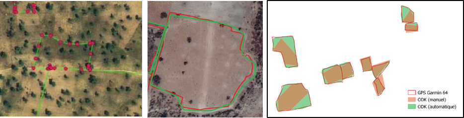
The first three criteria of the EO-based quality control concern the technical suitability of in situ data for EO applications. Typically, surveyors record GPS coordinates for household localization, crop observation placement, or field area measurement. Requirements for geospatial analysis include ensuring the topological soundness of spatial features, which involves verifying polygon closure, identifying duplicate points, and resolving polygon overlaps (Figure 9.1).

Figure 9.1: Quality control of geospatial features and their coordinates. Examples acquired during the FAO EOStat project in Senegal from left to right: polygon recorded as points sequence instead of a closed polygon, polygon overlap detected and solved, and benchmarking of various protocols and devices (tablet with integrated GPS versus Garmin receiver) to record field boundaries.

9.6 Measuring Spatial Precision of Field Plot Boundaries

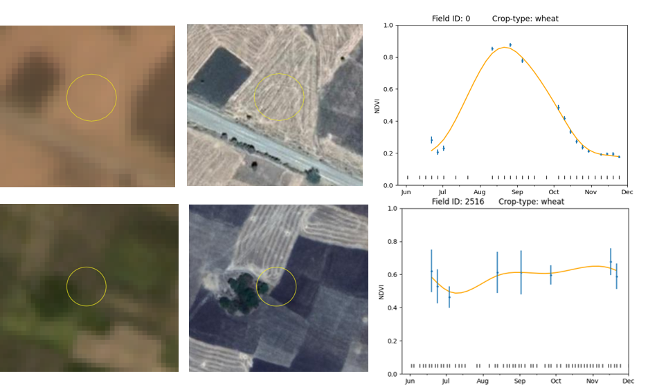
The last three criteria of the EO-based quality control rely on satellite imagery analysis. The spatial precision of field plot boundaries requires visual image interpretation of high spatial resolution imagery that aligns with the survey timeframe. This type of control usually involves overlaying the plotted polygons onto frequent data, such as monthly cloud-free surface reflectance base maps. Figure 9.2 shows a good-quality sample that aligns well with a cultivated field, whereas the second sample area covers multiple fields and some trees. The ideal situation is to use high-resolution images to visually check samples and plot boundaries and then classify the areas with lower spatial resolutions. A possible situation is to use 4.8-meter Planet monthly reflectance maps for sample quality control and 10-meter Sentinel-2 images for classification.

From an EO perspective, assessing sample quality requires time series from satellites such as Sentinel-2 for the growing season. Open-source platforms such as Sen4Stat and Sen2Agri toolbox [4] allow processing of all Sentinel-2 satellite images acquired along the season. One quantitative indicator of sample purity is the NDVI standard deviation (Figure 9.2, right plot) computed from the values of cloud-free satellite observations.

Figure 9.2: Cloud-free Planet monthly base map images (left) and very high-resolution imagery (middle) overlaid with point observation expected to be representative of a circle area (radius of 20 m), as reported by the 2020 wheat rust survey in Ethiopia (Blasch et al., 2022). Plots highlight expected and unexpected NDVI profiles and the associated standard deviation for a homogeneous wheat field derived from the Sentinel-2 time series during the surveyed season..

9.7 Using NDVI Temporal Profiles to Assess Crop Phenology

The last EO-based requirement is the most difficult to address. We assume that crops of the same type, grown in the same agro-climatic zone, have similar planting and growing cycles. Analysing NDVI profiles across all crop samples strengthens crop label confidence. Atypical growth patterns (e.g., varied planting/cycle length or lack of growth) indicate potential mislabeling or mislocated samples. These samples need more scrutiny before they can be deemed usable.

Consider Ethiopia’s diverse crop cycles in Figure 9.3. Temporal profiles for barley, fava beans, and teff show outliers indicating marginal sample quality. The different NDVI profiles for maize samples reveal that a significant portion underwent a double cropping cycle within the observation period. Since the first crop cycle delayed planting, the sample population needs to be divided appropriately using clustering methods. The complexity of the wheat cropping cycle is heightened by sowing dates and varietal differences affecting cycle length. Thus, EO quality control aims to reject unsuitable samples for model calibration and output validation. Subsequent EO-derived results, like crop type maps, area estimates, and yield forecasts, critically depended on this quality control process.

knitr::include_graphics("./images//th_design_frames/QA_plot_Ethiopia.png")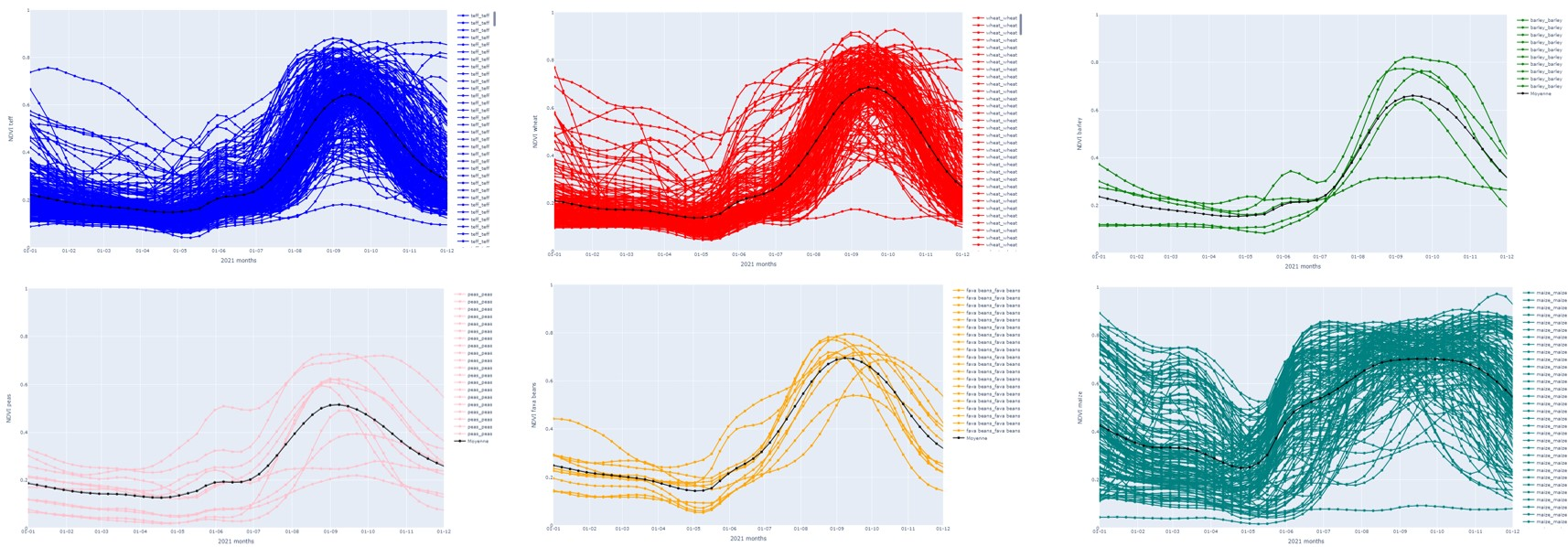

Figure 9.3: NDVI temporal profiles interpolated from cloud-free Sentinel-2 multispectral images acquired along the observation period. Each colour curve corresponds to a sample for a given crop, while the black curve is the average NDVI value of all samples for this crop. Teff is blue, wheat is red, barley is light green, peas are pink, fava beans are orange, and maise is dark green. The CIMMYT provided these samples in the framework of the ESA Sen4Rust partnership.

9.8 Summary

In this chapter, we provide recommendations for National Statistical Offices (NSO) to design in situ data collection campaigns that benefit both conventional statistics and EO-based assessments. Following these guidelines will increase the accuracy of EO-based land use classification.

References

[1]

C. Carletto, A. Dillon, and A. Zezza, “Agricultural Data Collection to Minimize Measurement Error and Maximize Coverage,” Global Poverty Research Lab, Working {{Paper}} 21-108, 2021.

[2]

W. G. Cochran, Sampling techniques. John Wiley & Sons, Ltd, 1977.

[3]

J. Delincé, “The cost-effectiveness of remote sensing in agricultural statistics,” J. Delincé, Ed. Rome: Handbook of the Global Strategy to improve Agricultural; Rural Statistics (GSARS), 2017.

[4]

P. Defourny et al., “Near real-time agriculture monitoring at national scale at parcel resolution: Performance assessment of the Sen2-Agri automated system in various cropping systems around the world,” Remote Sensing of Environment, vol. 221, pp. 551–568, 2019, doi: 10.1016/j.rse.2018.11.007.